An Introduction to MATLAB: Basic Operations
Contents
MATLAB is a programming language that is very useful for numerical simulation and data analysis. The following tutorials are intended to give you an introduction to scientific computing in MATLAB.
Lots of MATLAB demos are available online at
http://www.mathworks.com/academia/student_center/tutorials/launchpad.html
You can work through these at your leisure, if you want. Everything you need for EOS 225 should be included in the following tutorials.
Arithmetic Operations and Functions
At its simplest, we can use MATLAB as a calculator. Type
3+2
What do you get?
3+2
ans =

     5
Type
3*7
What do you get?
3*7
ans =

    21
Can also do more complicated operations, like taking exponents: for "3 squared" type
3^2
3^2
ans =

     9
For "two to the fourth power" type
2^4
2^4
ans =

    16
"Scientific notation" is expressed with "10^" replaced by "e" - that is, 10^7 is written 1e7 and 2.15x10^-3 is written 2.15e-3. For example:
1.5e-2
ans =

    0.0150
2e-3 * 1000
ans =

     2
MATLAB has all of the basic arithmetic operations built in:
         +   addition
         -   subtraction
         *   multiplication
         /   division (a/b = "a divided by b")
         ^   exponentiation
as well as many more complicated functions (e.g. trigonometric, exponential):
         sin(x)  sine of x (in radians)
         cos(x)  cosine of x (in radians)
         exp(x)  exponential of x
         log(x)  base e logarithm of x (normally written ln)
The above are just a sample - MATLAB has lots of built-in functions.
When working with arithmetic operations, it's important to be clear about the order in which they are to be carried out. This can be specified by the use of brackets. For example, if you want to multiply 5 by 2 then add 3, we can type
(5*2)+3
ans =

    13
and we get the correct value. If we want to multiply 5 by the sum of 2 and 3, we type
5*(2+3)
ans =

    25
and this gives us the correct value. Carefully note the placement of the brackets. If you don't put brackets, Matlab has its own built in order of operations: multiplication/division first, then addition/subtraction. For example:
5*2+3
ans =

    13
gives the same answer as (5*2)+3. As another example, if we want to divide 8 by 2 and then subtract 3, we type
(8/2)-3
ans =

     1
and get the right answer. To divide 8 by the difference between 2 and 3, we type
8/(2-3)
ans =

    -8
and again get the right answer. If we type
8/2-3
ans =

     1
we get the first answer - the order of operations was division first, then subtraction.
In general, it's good to use brackets - they invovle more typing, and may make a computation look more cumbersome, but they help reduce ambiguity regarding what you want the computation to do.
This is a good point to make a general comment about computing. Computers are actually quite stupid - they do what you tell them to, not what you want them to do. When you type any commands into a computer program like MATLAB, you need to be very careful that these two things match exactly.
You can always get help in MATLAB by typing "help". Type this alone and you'll get a big list of directories you can get more information about - which is not always too useful. It's more useful to type "help" with some other command that you'd like to know more about. E.g.:
help sin
 SIN    Sine of argument in radians.
    SIN(X) is the sine of the elements of X.

    See also ASIN, SIND, SINPI.

    Documentation for sin
       doc sin

    Other functions named sin

       codistributed/sin    dlarray/sin    gpuArray/sin    sym/sin
help atan
 ATAN   Inverse tangent, result in radians.
    ATAN(X) is the arctangent of the elements of X.

    See also ATAN2, TAN, ATAND, ATAN2D.

    Documentation for atan
       doc atan

    Other functions named atan

       codistributed/atan    gpuArray/atan    sym/atan
You can get a list of all the built-in functions by typing
help elfun
  Elementary math functions.

  Trigonometric.
    sin         - Sine.
    sind        - Sine of argument in degrees.
    sinh        - Hyperbolic sine.
    asin        - Inverse sine.
    asind       - Inverse sine, result in degrees.
    asinh       - Inverse hyperbolic sine.
    cos         - Cosine.
    cosd        - Cosine of argument in degrees.
    cosh        - Hyperbolic cosine.
    acos        - Inverse cosine.
    acosd       - Inverse cosine, result in degrees.
    acosh       - Inverse hyperbolic cosine.
    tan         - Tangent.
    tand        - Tangent of argument in degrees.
    tanh        - Hyperbolic tangent.
    atan        - Inverse tangent.
    atand       - Inverse tangent, result in degrees.
    atan2       - Four quadrant inverse tangent.
    atan2d      - Four quadrant inverse tangent, result in degrees.
    atanh       - Inverse hyperbolic tangent.
    sec         - Secant.
    secd        - Secant of argument in degrees.
    sech        - Hyperbolic secant.
    asec        - Inverse secant.
    asecd       - Inverse secant, result in degrees.
    asech       - Inverse hyperbolic secant.
    csc         - Cosecant.
    cscd        - Cosecant of argument in degrees.
    csch        - Hyperbolic cosecant.
    acsc        - Inverse cosecant.
    acscd       - Inverse cosecant, result in degrees.
    acsch       - Inverse hyperbolic cosecant.
    cot         - Cotangent.
    cotd        - Cotangent of argument in degrees.
    coth        - Hyperbolic cotangent.
    acot        - Inverse cotangent.
    acotd       - Inverse cotangent, result in degrees.
    acoth       - Inverse hyperbolic cotangent.
    hypot       - Square root of sum of squares.
    deg2rad     - Convert angles from degrees to radians.
    rad2deg     - Convert angles from radians to degrees.

  Exponential.
    exp         - Exponential.
    expm1       - Compute exp(x)-1 accurately.
    log         - Natural logarithm.
    log1p       - Compute log(1+x) accurately.
    log10       - Common (base 10) logarithm.
    log2        - Base 2 logarithm and dissect floating point number.
    pow2        - Base 2 power and scale floating point number.
    realpow     - Power that will error out on complex result.
    reallog     - Natural logarithm of real number.
    realsqrt    - Square root of number greater than or equal to zero.
    sqrt        - Square root.
    nthroot     - Real n-th root of real numbers.
    nextpow2    - Next higher power of 2.

  Complex.
    abs         - Absolute value.
    angle       - Phase angle.
    complex     - Construct complex data from real and imaginary parts.
    conj        - Complex conjugate.
    imag        - Complex imaginary part.
    real        - Complex real part.
    unwrap      - Unwrap phase angle.
    isreal      - True for real array.
    cplxpair    - Sort numbers into complex conjugate pairs.

  Rounding and remainder.
    fix         - Round towards zero.
    floor       - Round towards minus infinity.
    ceil        - Round towards plus infinity.
    round       - Round towards nearest integer.
    mod         - Modulus (signed remainder after division).
    rem         - Remainder after division.
    sign        - Signum.
Variables In MATLAB
MATLAB can be used like a calculator - but it's much more. It's also a programming language, with all of the basic components of any such language.
The first and most basic of these components is one that we use all the time in math - the variable. Like in algebra, variables are generally denoted symbolically by individual characters (like "a" or "x") or by strings of characters (like "var1" or "new_value").
An essential difference between the variable concept in algebra and in MATLAB is that: in algebra, a variable denoted by a letter (or group of letters) is a placeholder for an unknown or variable quantity, while in MATLAB it is a symbolic name given to a specified value (or set of values).
In class we've distinguished between variables and parameters - but denoted both of these by characters. MATLAB doesn't make this distinction - any numerical quantity given a symbolic "name" is a "variable".
How do we assign a value to a variable? Easy - just use the equality sign. For example
a =

     3
a =
3
sets the value 3 to the variable a. As another example
b =

     2
b =
2
sets the value 2 to the variable b. We can carry out mathematical operations with these variables: e.g.
a+b
ans =

     5
a*b
ans =

     6
a^b
ans =

     9
exp(a)
ans =

   20.0855
Although the operation of setting a value to a variable looks like an algebraic equality like we use all the time in math, in fact it's something quite different. The MATLAB statement
a =

     3
should not be interpreted as "a is equal to 3". It should be interpreted as "take the value 3 and assign it to the variable a". This difference in interpretation has important consequences. In algebra, we can write a = 3 or 3 = a -- these are equivalent. The = symbol in MATLAB is not symmetric - the command
a = b
should be interpreted as "take the value of b and assign it to the variable a" - there's a single directionality. And so, for example, we can type
a =

     3
a =
3
with no problem, if we type
3=a
we get an error message (try it!). The value 3 is fixed - we can't assign another number to it. It is what it is.
Another consequence of the way that the = operator works is that a statement like
a = a+1
makes perfect sense. In algebra, this would imply that 0 = 1, which is of course nonsense. In MATLAB, it means "take the value that a has, add one to it, then assign that value to a". This changes the value of a, but that's allowed. For example, type:
a = 3
a =
3
then
a = a+1
a =

     4
First a is assigned the value 3, then (by adding one) it becomes 4.
There are some built in variables; one of the most useful is pi:
pi
ans =

    3.1416
We can also assign the output of a mathematical operation to a new variable: e.g.
b = a*exp(a)
b =

  218.3926
b
b =

  218.3926
If you want MATLAB to just assign the value of a calculation to a variable without telling you the answer right away, all you have to do is put a semicolon after the calculation:
b = a*exp(a);
Being able to use variables is very convenient, particularly when you're doing a multi-step calculation with the same quantity and want to be able to change the value. For example:
a = 1;
b = 3*a;
c = a*b^2;
d = c*b-a;
d
d =

    26
Now say I want to do the same calculation with a = 3; all I need to do is make one change
a = 3;
b = 3*a;
c = a*b^2;
d = c*b-a;
How does this make things any easier? Well, it didn't really here - we still had to type out the equations for b, c, and d all over again. But we'll see that in a stand-alone computer program it's very useful to be able to do this.
In fact, the sequence of operations above is an example of a computer program. Operations are carried out in a particular order, with the results of earlier computations being fed into later ones.
It is very important to understand this sequential structure of programming. In a program, things happen in a very particular order: the order you tell them to have. It's very important to make sure you get this order right. This is pretty straightforward in the above example, but can be much more complicated in more complicated programs.
Any time a variable is created, it's kept in memory until you purposefully get rid of it (or quit the program). This can be useful - you can always use the variable again later. It can also make things harder - for example, in a long program you may try using a variable name that you've already used for another variable earlier in the program, leading to confusion.
It can therefore be useful sometimes make MATLAB forget about a variable; for this the "clear" command is used. For example, define
b = 3;
Now if we ask what b is, we'll get back that it's 3
b
b =
3
Using the clear command to remove b from memory
clear b
now if we ask about b
b
we get the error message that it's not a variable in memory - we've succeeded in getting rid of it. To get rid of everything in memory, just type
clear all
Arrays
An important idea in programming is that of an array (or matrix). This is just an ordered sequence of numbers (known as elements): e.g.
M = [1, 22, -0.4]
is a 3-element array in which the first element is 1, the second element is 22, and the third element is -0.4. These are ordered - in this particular array, these numbers always occur in this sequence - but in general, there isn't any constraint on the values the elements can have or the order they take. That is - in an array, numbers don't have to increase or decrease or anything like that. The numbers can be integers or rational numbers, or positive or negative. The numbers that are present and the order in which they occur define the array.
While the elements of the array can be any kind of number, their positions are identified by integers: there is a first, a second, a third, a fourth, etc. up until the end of the array. We can indicate the position of the array using bracket notation: in the above example, the first element is
M(1) = 1
the second element is
M(2) = 22
and the third element is
M(3) = -0.4.
These integers counting off position in the array are known as "indices" (singular "index").
All programming languages use arrays, but MATLAB is designed to make them particularly easy to work with (the MAT is for "matrix"). To make the array above in MATLAB all you need to do is type
M = [1 22 -0.4]
M =

    1.0000   22.0000   -0.4000
Then to look at individual elements of the array, just ask for them by index number:
M(1)
ans =

     1
M(2)
ans =

    22
M(3)
ans =

   -0.4000
We can also ask for certain ranges of an array, using the "colon" operator. For an array M we can ask for element i through element j by typing
M(i:j)
E.g.:
M(1:2)
ans =

     1    22
M(2:3)
ans =

   22.0000   -0.4000
If we want all elements of the array, we can type the colon on its own
M(:)
ans =

    1.0000
   22.0000
   -0.4000
We can also use this notation to make arrays with a particular structure. Typing
M = a:b:c
makes an array that starts with first element
M(1)=a
and increases with increment b:
M(2) = a+b
M(3) = a+2b
M(4) = a+3b
etc.
The array stops at the largest value of N for which M(N) has not gone beyond c.
Example 1:
M = 1:1:3
M =

     1     2     3
The array starts with 1, increases by 1, and ends at 3
Example 2:
M = 1:.5:3
M =

    1.0000    1.5000    2.0000    2.5000    3.0000
The array starts at 1, increases by 0.5, and ends at 3
Example 3:
M = 1:.6:3
M =

    1.0000    1.6000    2.2000    2.8000
Here the array starts at 1, increases by 0.6, and ends at 2.8 - because making one more step in the array would make the last element bigger than 3.
Example 4:
M = 3:-.5:1
M =

    3.0000    2.5000    2.0000    1.5000    1.0000
This kind of array can also be decreasing.
If the increment size b isn't specified, a default value of 1 is used:
M = 1:5
M =

     1     2     3     4     5
That is, the array a:c is the same as the array a:1:c
It is important to note that while the elements of an array can be any kind of number, the indices must be positive integers (1 and bigger). Trying non-positive or fractional integers will result in an error message: try typing
M(-1)
M(10.5)
Each of the elements of an array is a variable on its own, which can be used in a mathematical operation. E.g.:
M(1)+M(3)
ans =

     4
M(2)*M(3)
ans =

     6
The array itself is also a kind of variable - an array variable. You need to be careful with arithmetic operations (addition, subtraction, multiplication, division, exponentiaion) when it comes to working with entire arrays - these things can be defined, but they have to be defined correctly. We'll look at this later.
In MATLAB, when most functions are fed an array as an argument they give back an array of the function acting on each element. That is, for the function f and the array M,
g = f(M)
is an array such that
g(i) = f(M(i)).
E.g.
a = 0:4;
b = exp(a)
b =

    1.0000    2.7183    7.3891   20.0855   54.5982
Plotting
Let's define two arrays of the same size
a = 1:5;
b = exp(a);
Now type
plot(a,b)
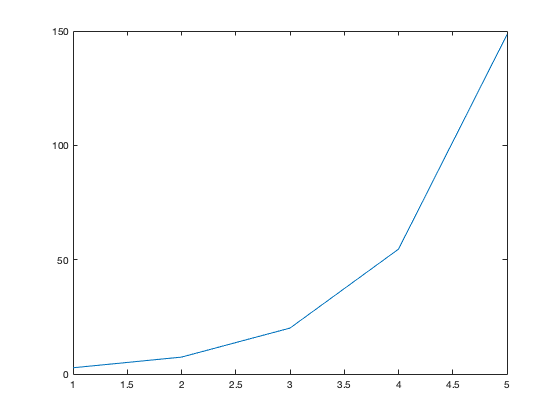
and what we get is a plot of the array a versus the array b - in this case, a discrete version of the exponential function exp(x) over the range x=1 to x=5.
We can plot all sorts of things: the program
a = 0:.01:5;
b = cos(2*pi*a);
plot(a,b)
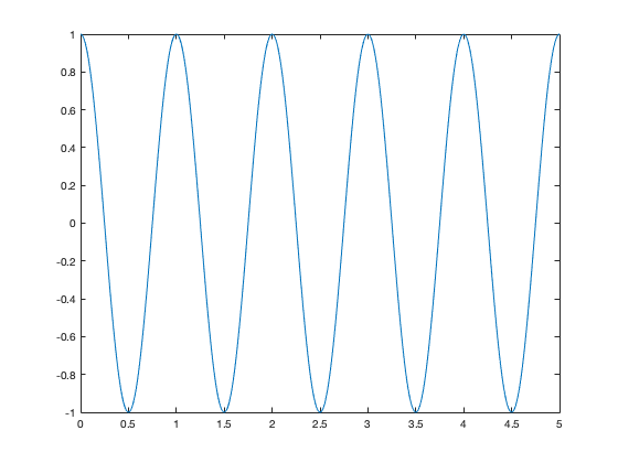
sets the variable a as a discretisation of the range from x=0 to x=5 with step 0.1, defines b as the cosine of 2 pi x over that range, and then plots a agaist b - showing us the familiar sinusoidal waves.
We can also do all sorts of things with plots - stretch them vertically and horizontally, flip them upside down, give them titles and label the axes, have multiple subplots in a single plot ... but we'll come to these various features as we need them.
One particularly useful thing we can do with plotting is to find approximate solutions to equations that can't be solved analytically: for example, the equation ln(x) = x-2. You can exponentiate both sides, but then you just end up with x = exp(x-2) - which also can't be solved analytically.
Graphical solutions of the equation f(x) = g(x) are based on the fact that a solution is any value of x for which f(x) and g(x) take the same value. This equation can be written as
0 = f(x)-g(x)
so another way of thinking about a solution to the original equation is that it is any value of x for which f(x)-g(x) takes the value zero.
To solve an equation graphically, all we have to do is plot f(x)-g(x) and see where it takes the value of zero. The trick here is making sure that we plot f(x)-g(x) over the right range of values to include any zeros (in general there will be more than one). Determining this range can be a process of trial and error.
Going back to our earlier example: we want to solve ln(x)=x-2. In other words, we want to find values of x so that 0 = x-2-ln(x). Remember that ln(x) is only defined for x>0, so when plotting we don't need to consider x<=0. Let's make the plot from x = 0.1 to x = 5 in steps of 0.1 (remembering that in MATLAB the command for the natural logarithm is "log")
x = .1:.1:5;
plot(x,x-2-log(x))
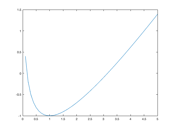
From the plot, it is clear that the curve x-2-ln(x) crosses zero at two points in the range of x values being displayed. Zooming into the plot (using the magnifying glass icon above the plot frame) allows us to read off that these zero values are at approximately x = 0.18 and x = 3.14. From this figure alone, we cannot conclude that there are not other zeros (although with a more detailed investigationof the functions ln(x) and x-2, we can make this argument). To confirm we have found approximate solutions of the equation, we compute
.18-2
ans =

   -1.8200
log(.18)
ans =

   -1.7148
and
3.14-2
ans =

    1.1400
log(3.14)
ans =

    1.1442
These pairs of values aren't exactly the same - but they're very close, and we could get them even closer if we zoomed in more on the plot to get a better estimate of where the curve crosses zero.
Arithmetic Operations on Arrays
Arithmetic operations (addition, subtraction, multiplication, division) between an array and a scalar (a single number) are straightforward. If we add an array and a scalar, every element in the array is added to that scalar: the ith element of the sum of the array M and the scalar a is M(i)+a.
M = [1 3 -.5 7];
M2 = M+1
M2 =

    2.0000    4.0000    0.5000    8.0000
Similarly, we can subtract, multiply by, and divide by a scalar.
M3 = 3*M
M3 =

    3.0000    9.0000   -1.5000   21.0000
M4 = M/10
M4 =

    0.1000    0.3000   -0.0500    0.7000
It's even possible to add, subtract, multiply and divide arrays with other arrays - but we have to be careful doing this. In particular, we can only do these things between arrays of the same size: that is, we can't add a 5-element array to a 10-element array.
If the arrays are the same size, these arithmetic operations are straightforward. For example, the sum of the N-element array a and the N-element array b is an N-element array c whose ith element is
c(i) = a(i)+b(i)
For example:
a = [1 2 3];
b = [2 -1 4];
c = a+b;
c
c =

     3     1     7
That is, addition is element-wise (element by element). It's just the same with subtraction.
d = a-b;
d
d =

    -1     3    -1
With multiplication we use a somewhat different notation. Mathematics defines a special kind of multiplication between arrays - matrix multiplication - which is not what we will consider in this course. However, it's what MATLAB thinks you're doing if you use the * sign between arrays. To multiply arrays element-wise (like with addition), we need to use the .* notation (note the " . " before the " * "):
f = a.*b;
f
f =

     2    -2    12
The result is an array f whose ith element is the product of the ith element of a with the ith element of b:
f(i) = a(i)*b(i).
Similarly, to divide, we don't use /, but rather ./
g = a./b;
g
g =

    0.5000   -2.0000    0.7500
(once again, note the dot). As we'll see over and over again, it's very useful to be able to carry out arithmetic operations between arrays.
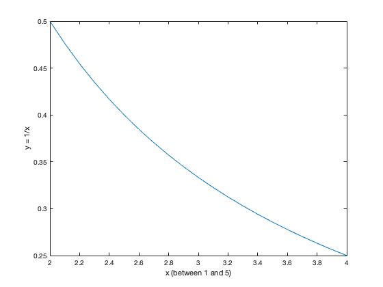
For example, say we want to make a plot of x versus 1/x between x = 2 and x = 4. Then we can type in the program
x = 2:.1:4;
y = 1./x;
plot(x,y)
xlabel('x');
ylabel('y');
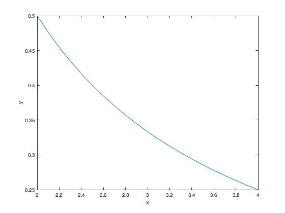
Note how we put the labels on the axes - using the commands xlabel and ylabel, with the arguments 'x' and 'y'. Because the arguments are character strings - not numbers - they need to be in single quotes. The axis labels can be more complicated, e.g.
xlabel('x (between 1 and 5)')
ylabel('y = 1/x')
We haven't talked yet about how to exponentiate an array. To take the array M to the power b element-wise, we type M.^b Note again the "." before the "^" in the exponentiation. As an example
x = [1 2 3 4];
y = x.^2
y =

     1     4     9    16
We can also take a scalar to the power of an array:
x = [1 2 3 4];
y = 2.^x
y =

     2     4     8    16
As another example, we can redo the earlier program:
x = 2:.1:4;
y = x.^(-1);
plot(x,y)
xlabel('x');
ylabel('y');

Note that we put the "-1" in brackets - this makes sure that the minus sign associated with making the exponent negative is applied before the "^" of the exponentiation. In this case, we don't have to do this - but when programming it doesn't hurt to be as specific as possible.
These are the basic tools that we'll need to use MATLAB. Subsequent tutorials will cover other aspects of writing a program - but what we've talked about above forms the core. Everything that follows will build upon the material in this tutorial.
Exercises
The following exercises will use the tools we've learned above and are designed to get you thinking about programming.
In writing your programs, you'll need to be very careful to think through:
(1) what is the goal of the program (what do I need it to do?)
(2) what do I need to tell MATLAB?
(3) what order do I need to tell it in?
It might be useful to sketch the program out first, before typing anything into MATLAB. It can even be useful to write the program out on paper first and walk through it step by step, seeing if it will do what you think it should.
Exercise 1
Multiply 3 by 8 and divide this product by the difference between 13 and 7.
Exercise 2
Compute
  (a) log(5^2)
  (b) 2 log(5)
Compare the values of these calculations.
Exercise 3
Remember the expression for the amount of U238 remaining after n billion years have elapsed: U(n) = (1-alpha)^n U(0).
If at t=0 a sample has 2nmol of U238, how much remains after 5 billion years has elapsed?
Exercise 4
Solve the equation
0.2 = sin(x)
for -pi/2 < x < pi/2. Do this in two ways - one using a builit-in MATLAB function, and the other using a graphical solution.
Exercise 5
Solve the equation
exp(x) = x+2
graphically. Note that there may be more than one solution.
Exercise 6
Plot the following functions:
(a) y = 3x+2 with x = 0, 0.25, 0.5, ...., 7.75, 8
(b) y = exp(-x^2) with x = 0, 0.1, 0.2, ..., 2
(c) y = cos(x) with x = 0,pi/10,2*pi/10, ..., 2*pi
(d) y = (ln(exp(x)))^-1 with x = 1, 1.5, 2, ..., 4
Exercise 7
Carry out the following calculations:
(a) Find the square root of 387 in two different ways.
(b) In a single line of code, find the square roots of the integers from 3 to 15. Do this in two ways.
(c) Repeat (b) for the even integers between 3 and 15.
Exercise 8
Solve the equation
x^2 = 5x-6
in two different ways - first finding the solution by hand (e.g. using the quadratic formula) and then using a graphical solution.
Exercise 9
Plot the function
h(t) = 2[3exp(2t)-exp(-2t)]/[3exp(2t)+exp(-2t)]
from t=0 to t=6.
Exercise 10
Plot the function
y(x) = x + x exp(-1/x)
from x = 0 to x=5.
Exercise 11
You have a lump of U238 of mass 10g. Plot the mass of U238 as a function of time for the next 6 billion years. (Recall the discussion in Section 1.1 of the notes).
Exercise 12
C14 has a 1/2-life of 5730 years. A sample is measured to have 10 mg of C14. Plot the mass of C14 as a function of time from 20,000 years in the past to 20,000 years in the future. Remember that if T is the half-life and C(t) is the amount of C14 at time t, then by definition of the half life:
C(t) = C(0) 2^(-t/T)
Exercise 13
A mountain range has a tectonic uplift rate of 1 mm/yr and erosional timescale of 1 million years. If the mountain range starts with a height h(0) = 0 at time t = 0, write a program that predicts and plots the height h(t) at t=0, t=1 million years, t=2 million years, t=3 million years, t=4 million years, and t=5 million years (neglecting isostatic effects). Label the axes of this plot, including units.
Exercise 14
Repeat Exercise 13 in the case that the erosional timescale is 500,000 years.
Exercise 15
Repeat Exercise 13 in the case that the tectonic uplift rate is 2 mm/yr.
Exercise 16
From observations of an orogen you know the following information:
h(0) = 500m
h(t1) = 750m at t1 = 10^6 yr
beta = 0.5 mm/yr
Assuming that the erosion rate is linearly proportional to the elevation find the value of the erosional timescale tau_e. (This requires a graphical solution of an equation).
Exercise 17
Repeat Exercise 16 in the situation that you do NOT know the value of h(0) but you know that h(t2) = 1025m at t2 = 3x10^6 yr. Confirm that this calculation gives you the value for h(0) from Exercise 16.