An Introduction to MATLAB: For Loops and M-Files
Contents
The For Loop
We will now consider our next example of fundamental concepts in computer programming: the for loop (more generally, ``iteration'').
We talked in class about an example of an iterative calculation - radioactive decay. Starting with some amount of U238, we know that each billion years we lose a fraction alpha, that is,
U(2) = (1-alpha)U(1)
U(3) = (1-alpha)U(2) = [(1-alpha)^2] U(1)
U(4) = (1-alpha)U(3) = [(1-alpha)^3] U(1)
and so on. To predict U(n), we start with U(1) and iteratively multiply by the factor 1-alpha. How do we do this in MATLAB?
In this case, we have a formula predicting U(n) from U(1), so we can just use the exponentiation function - we know how to take the nth power of some factor. In general, iterative calculations don't admit closed-form expressions for the nth step in terms of the first. But there's another way to do the calculation - using the for loop.
Before talking about the for loop, it's worth emphasising the following fact: computers were invented to do exactly this kind of computation. Many important applications involve doing similar calculations repeatedly, with each step making use of the results of the previous step (that is, using iterations). This can be incredibly tedious to do by hand - and errors can creep in, through carelessness or boredom. Computers don't get bored - they'll happily do the same thing over and over again. What we're learning now is at the heart of how computers work.
Going back to our radioactive decay example: to compute the mass of U238 present after 3 billion years have elapsed from some initial time, we could just type out the sequence of calculations above by hand, one after the other. With the initial mass
U(1) = 0.5 kg:
we can write
clear all
alpha = 0.143;
U(1) = 0.5;
U(2) = (1-alpha)*U(1);
U(3) = (1-alpha)*U(2);
U(4) = (1-alpha)*U(3);
U
U =

    0.5000    0.4285    0.3672    0.3147
Note that we've had to type the same thing over and over: take the result of the previous calculation and multiply by the same factor. This is a nuisance, and impossible in practice for bigger calculations - what if you had to go out to n=50? What are the chances you'd make a typo? Pretty large in fact ...
Before carrying on: note the indices of the array U. U(1) is the first element of U - corresponding to the time n=0 in the notation of Section 1.1 of the notes. Remember that the indices of the array must be positive integers. U(1) corresponds to the amount of U238 at the first time considered - which in this case is the initial amount, at "time" n=0. Similarly, U(2) is the amount after the first billion years has elapsed, U(3) is the amount after the second billion years, etc.
The for loop provides a much more efficient way of calculating U(4) calculation:
clear all
alpha = 0.143;
U(1) = 0.5;
for k=2:4
    U(k) = (1-alpha)*U(k-1);
end
U
U =

    0.5000    0.4285    0.3672    0.3147
We get the same answer, but with a more compact program.
Note the structure of the for loop: we only have to tell MATLAB once how the iteration works, from step k - 1 to step k. But what is k? It is a counter of where we are in the iteration. If we start with k = 2, then we get the step from k - 1 = 1 to k = 2 - that is, from U(1) to U(2). With k = 3, we get the step from k - 1 = 2 to k = 3 - that is, from U(2) to U(3) - and so on and so forth. This process stops when k takes the value of 4. As we will see, not all iterations involve taking the value from a previous step and using it in the present step - although this will often be the case.
The range of steps to be taken is listed at the top of the for loop - we told MATLAB to run k from 2 to 4 (in increments of 1, the default for the : operator).
This sequence of steps can be represented visually as a flow chart:
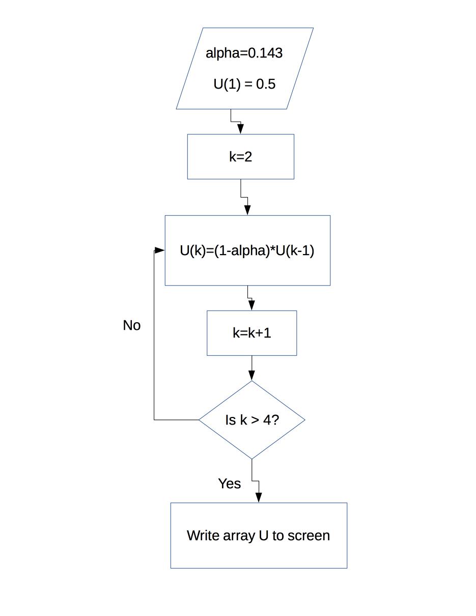
The program begins by defining the parameter alpha and the value of U(1). Starting with k = 2, it then computes U(k) from U(k-1). After doing this, the value of k is increased by 1. When k exceeds 4, the iteration stops and the array is written to the screen.
At each iteration, MATLAB does everything between the "for" and "end" statements in the loop. In the above example, that's a single calculation - but it doesn't have to be. The "end" command is very important here - it tells MATLAB where to end the sequence of commands making up the for loop.
For example, say we want MATLAB to compute the square, cube, and fourth power of all integers between 4 and 8. We can write the program:
clear all
x = 4:8;
for k=1:5
    s(k) = x(k)^2;
    c(k) = x(k)^3;
    f(k) = x(k)^4;
end
s
c
f
s =

    16    25    36    49    64


c =

    64   125   216   343   512


f =

         256         625        1296        2401        4096
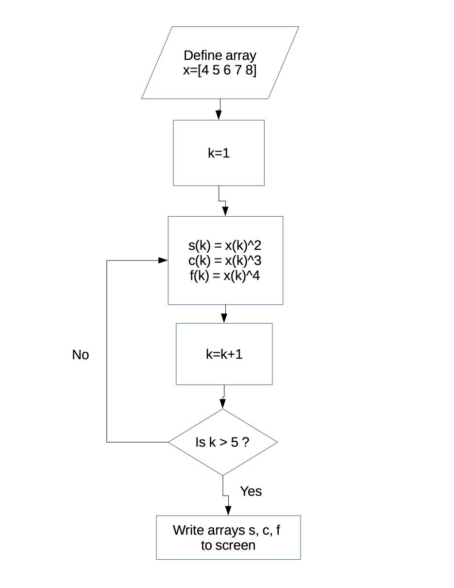
The counter k which keeps track of where we are in the loop starts at one, and increases by one until it reaches 5. The counter starts at k=1, corresponding to the first element in the array x (which is x(1)=4) and ends with the value k=5, corresponding to the last element (which is x(5)=8). At each step, each of the square, cube, and fourth power are computed and stored in different arrays. Note that here the output of the kth step is saved in the kth element of each array.
This program can be represented graphically by the following flow chart:
We can make the sequence of commands between the "for" and "end" as complicated as we want - we can even have other for loops inside a for loop (called "nesting"). But the basic idea is just this: do a perscribed sequence of steps, over and over again, for a pre-determined number of times.
The counter k is a variable itself. In fact, the counter doesn't have to be called "k" - it can be called anything. For example, typing
clear all
x = 4:8;
for j=1:5
    s(j) = x(j)^2;
    c(j) = x(j)^3;
    f(j) = x(j)^4;
end
s
c
f
s =

    16    25    36    49    64


c =

    64   125   216   343   512


f =

         256         625        1296        2401        4096
gives exactly the same thing as with the counter called "k". The important thing to remember is not to give the counter the same name as another variable that you still want to use - particularly one you'll be modifying in the for loop. Anybody who's done much programming has spent many hours of their life debugging programs where that was the error.
Note that we could also get the desired results from the code above using the program
clear all
x = 4:8;
s = x.^2;
c = x.^3;
f = x.^4;
s
c
f
s =

    16    25    36    49    64


c =

    64   125   216   343   512


f =

         256         625        1296        2401        4096
The use of a for loop here isn't necessary - there is often more than one way to carry out the same calculation, using different coding tools.
In the earlier for loop example, computing the mass of uranium as a function of time, we used the value of the k-1 step to compute the value at the k step. We could also write the loop such that we use the value of the k step to get the value at k+1:
clear all
alpha = 0.143;
U(1) = 0.5;
for k=1:3
    U(k+1) = (1-alpha)*U(k);
end
U
U =

    0.5000    0.4285    0.3672    0.3147
The output of this program is exactly equal to that of the earlier one - because it is carrying out the same iteration, albeit written in a somewhat different form. Note that we have had to change the range of k values: as the first U value we are computing in the iteration is the second element of the array, then if we're identifying this step as going from k to k+1, we need the first value of k to be 1 so that k+1=2. If the last value of U we're going to calculate is the 4th element of the array, then the last value of k we need is 3 (so that k+1 = 4).
The increment in a for loop doesn't have to be 1; for example we can have
clear all
for j=2:2:8
    3*j
end
ans =

     6


ans =

    12


ans =

    18


ans =

    24
In this case, the counter j goes up in steps of 2. A for loop can have any increment (unlike array indices which must be positive integers).
The general structure of for loops can be expressed:
for (counter) = (start):(increment):(end)
(stuff to be done in for loop)
end
Let's go back to the radioactive decay example, and see how Figure 1.1 in the notes was made.
We want to see how U(t) changes from t=0 Ga to t=25 Ga , starting from U(0). If we define the ratio
r(t) = U(t)/U(0)
(where r is to be interpreted as a function of time - not as a MATLAB array) then from above we have the iteration
r(t) = (1-alpha)r(t-1)
with r(0) = 1 (where as written the argument of the function r is the time t=0). So if we write the program
clear all
alpha = 0.143;
t = 0:25;
r(1) = 1;
for k=2:26;
    r(k) = (1-alpha)*r(k-1);
end
plot(t,r)
xlabel('t (Ga)');
ylabel('U(t)/U(0)');
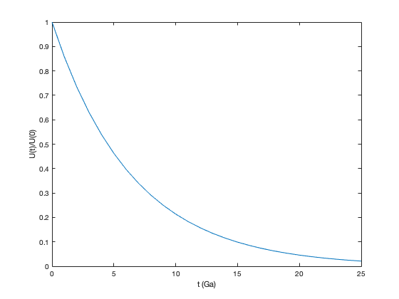
we get pretty much the plot in Figure 1.1 Note that because array indices must be positive, t = 0 corresponds to k=1 and t=25 Ga corresponds to k=26. In this MATLAB script, the quantity
r(k)
is not the value of r at the time k - it is the value of the kth element of the array r. If the kth element of the array r corresponds to the kth element of the array t, then in particular the first element of the array t (which has a value equal to 0) will correspond to the first element of the array r (which has a value equal to 1). When interpreting an expression, it is crucially important to remember if it is meant to represent algebra or computer code.
It would have been a lot of work to type out the iteration 25 times - for this reason, the for loop is an essential part of computer programming.
Note that the figure we got above isn't exactly Figure 1.1, which has a bunch of other stuff on it. In fact, Figure 1.1 was produced by the following code
clear all
t = 0:1:25;
alpha = .143;
U = (1-alpha).^t;
plot(t,U,'k','linewidth',2)
xlabel('t (Ga)','fontsize',24);
tmp=ylabel('U(t)/U(0)','fontsize',24);
set(gca,'fontsize',18);
hold on
plot(4.5,0.025,'^','markerfacecolor','k','markeredgecolor','k','markersize',18);
t2 = 0:.01:1;
plot(4.5*ones(size(t2)),t2,'--k')
hold off
text(5,.15,'Age of Earth','fontsize',15)
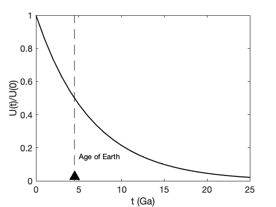
While we haven't talked about all the things you need to understand everything in the above code, it's still worth looking at. When programming, it's often useful to examine how other people have written code - it's often easier to learn by example, seeing how other people have done things, rather than trying to do everything from first principles. Searching online is also a valuable way of figuring out how to do something new in programming.
M-Files
Look at the previous piece of code - it's 13 lines long, with some fairly complicated bits. Typing this out fully each time you want to make this Figure would be tedious - and error-prone. Now imagine a weather prediction program, which might have millions of lines of code - there's no way this can be retyped in full every 6 hours to make a forecast.
Programming languages get around this by storing programs in separate computer files. In MATLAB, these are known as M-files and always end with the suffix .m ("dot-m"). When you have the M-file "sample_program.m", you can run it by simply typing
sample_program
on the command line (note that you don't include the suffix ".m" in what you type).
Working with M-files is crucial, particularly if there's a program you're going to use multiple times (and so don't want to have to retype it in full each time), if the program has complicated lines of code in which it's easy to make a typo, or if the program is very long.
Programming M-files is no harder than programming on the command line - you just type out the sequence of commands in the order that you want them executed (just like you would on the command line) and that's the order in which MATLAB carries them out.
To make a new M-file, click on "New Script" icon in the upper left of the MATLAB window. This will open a new text editor window - a window you can type your program in.
A nice thing about M-files is that they can include notes to yourself (and others) about what the M-file does, both overall and in particular places. These are called "comments", and anything on a line appearing after a percentage sign "%" is "commented out". That is, anything on that line following the "%" will appear in the M-file MATLAB won't pay any attention to it.
Now, type the following program into the text editor
% My test program
a = 3;
b = 2;
c = 1:4;
d = a*(c.^b);
plot(c,d);
Right now, this text hasn't been saved as a file - it's just sitting in the text editor, and can't be run by MATLAB. To be able to run the program, you'll need to save the M-file. To do this, press the "Save" icon above your script (to the left). This will give you a menu where you can pick what you'll call the file. Call this one
my_test_program.m
Now you can go to the MATLAB command window and at the command line type
my_test_program
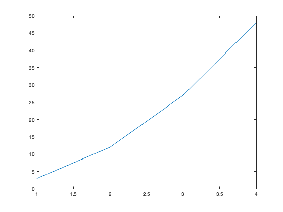
Up comes the plot of the array c against the array d. We can ask for the values of the array d
d
d =

     3    12    27    48
or of the variable b
b
b =

     2
It's all as if we'd typed each line in the command window. But here's one major advantage - say we want to look at the plot of c against d again, but now for the case that a = 4. If we'd typed each line in the command window, we'd have to go back and start typing them in again, right from the beginning. But we can go to the M-file and edit the first line to read
a = 4
instead. To run this new M-file, we first need to save it as a new file - using the "Save As" option under the "File" menu. Let's call this new file "my_test_program_2.m" Once the file is saved, we run the new M-file
my_test_program_2
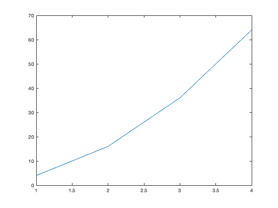
and get another plot, now for the value a=4.
These aren't very realistic examples so far. Let's consider working with Eqn. (2.10) for the growth of a mountain range under the influence of tectonic uplift and erosion (neglecting isostatic effects). To start with, we open a clean new text editor. Now type the following
% Orogeny example, Eqn. (2.10)
beta = 0.1e-3; %% m/yr
tau = 5e6; %% yr
h0 = 0; %% initial topgraphy zero
t = 0:1e5:25e6; %% time in steps of 100,000 years from t=0 to t=25^6 years
h = beta*tau + (h0-beta*tau)*exp(-t/tau);
plot(t/10^6,h/1e3)
xlabel('t (Ma)')ylabel('h (km)')Notice how the comments have been used to remind us what the units of different variables are. Now save this program under the name
orogony_example_1.m
Running this m-file gives the plot of h(t) against t:
orogeny_example_1
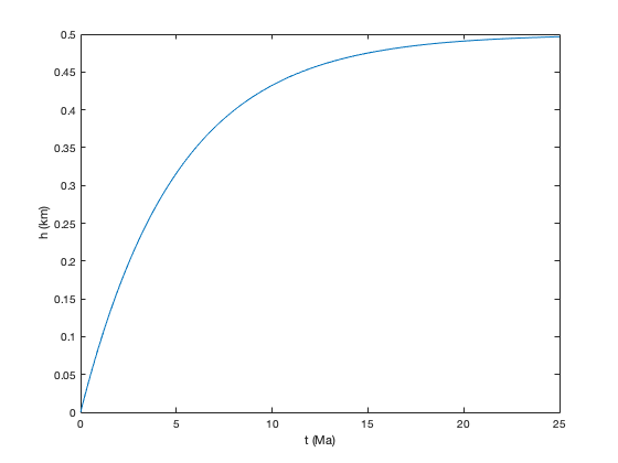
We see the familiar increase in h(t) with t, approaching the steady state value h_eq = 500 m.
Note the trick we've played in the plot: we didn't exactly plot t with h. Rather, we plotted t/1e6 with h/1e3. Because t is in years and h is in metres, doing this means that the plot's x-axis is in units of Ma (10^6 years) and the y-axis is in units of km (10^3 m) - as we've noted in the axis labels.
Whenever you work with dimensional quantities in MATLAB (or other programming languages) it is important to be careful with units. MATLAB has no idea of what the units of numbers in memory are - they're just numbers. If you enter the initial height of topography to be 10, MATLAB won't know if this is 10 m, 10 km, or 10 mm. When working with dimensional quantities, you have to decide at the start what units you are going to use - how are you going to measure length (m? mm? km? another length?), how you will measure time (seconds? hours? years? another length?), how you will measure mass, etc. You can use any units you want - but you have to be consistent with them in your calculations.
NxM Arrays
So far, we have only considered arrays with a single index. E.g.
M = [82 , -1.8 , 6]
for which
M(1) = 82
M(2) = -1.8
M(3) = 6
In fact, MATLAB allows arrays with more than one index. For the case of an array with two indices, you can think of it as a set of numbers arranged on a grid with rows and columns. E.g.
M =
1 3 -12
6 0.1 8
-0.3 7 12
4 -4 4
This array has 4 rows and 3 columns - so is called a 4x3 array. In general, an array with M rows and N columns is referred to as being MxN. The single-index arrays we've already talked about can be considered 1xN arrays.
You can think of the MxN array as a container with many small compartments (like an egg carton) arranged in a grid. Each compartment holds a number. Each compartment is also identified by a pair of numbers - the first indicates the row, the second the column. The numbers identifying the compartment (the indices) are both integers - counting rows (from the top) and columns (from the left) - but any kind of number can be IN the compartment. In MATLAB indices must take a value of one or greater.
We can look at individual elements of such an array. We use the notation:
M(i,j)
is the element of M in the ith row (counting from the top) and the jth column (counting from the left). In the example above
M(1,2) = 3
M(3,3) = 12
M(4,2) = -4
To put the above array into MATLAB, type the following in the command line:
M = [ 1 3 -12 ; 6 0.1 8 ; -0.3 7 12 ; 4 -4 4]
M =

    1.0000    3.0000  -12.0000
    6.0000    0.1000    8.0000
   -0.3000    7.0000   12.0000
    4.0000   -4.0000    4.0000
The array is entered row by row, separated by semicolons (you could use commas to separate the column values within a particular row, but you don't have to).
We can ask MATLAB for the values of individual array elements
M(1,2)
ans =

     3
M(3,3)
ans =

    12
M(4,2)
ans =

    -4
or for parts of whole rows or columns. For example
M(2:4,1)
ans =

    6.0000
   -0.3000
    4.0000
gives the elements in the first column from rows 2 through 4
M(3,1:2)
ans =

   -0.3000    7.0000
gives the elements in the columns 1 through 2 in row 3
M(:,2)
ans =

    3.0000
    0.1000
    7.0000
   -4.0000
gives all elements in column 2 and
M(3,:)
ans =

   -0.3000    7.0000   12.0000
gives all elements in row 3.
Such higher-dimensional arrays are useful for all sorts of things, as we'll see in the following example.
Let's compare the predictions made by the model of orogeny for different values of the initial topographic height h(0). Type the following into a new M-file:
% Orogeny example, Eqn. (2.10)
beta = 0.1e-3; %% m/yr
tau = 5e6; %% yr
h0 = [0 250 750 1000];
t = 0:1e5:25e6; %% time in steps of 100,000 years from t=0 to t=10^6 years
for k=1:length(h0)
h(k,:) = beta*tau + (h0(k)-beta*tau)*exp(-t/tau);
end
plot(t/10^6,h(1,:)/1e3,'r')
hold on
plot(t/10^6,h(2,:)/1e3,'g')
plot(t/10^6,h(3,:)/1e3,'b')
plot(t/10^6,h(4,:)/1e3,'k')
hold off
xlabel('t (Ma)')ylabel('h (km)')legend('0 m','250 m','750 m','1000 m')and save the M-file as
orogeny_example_2.m
Running this M-file:
orogeny_example_2
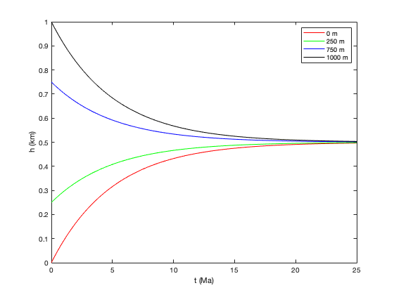
This plot has four curves h(t), one each for
h(0)=0 m
h(0)=250 m
h(0)=750 m
and
h(0)=1000 m.
Each curve approaches the steady state value as t increases: in those cases where the topography starts below the steady state value, h(t) increases with time; in those cases in which the topography starts below the steady state value, h(t) decreases with time.
Look at how we made this plot. First, we didn't define a single initial condition h(0) - we defined an array with four values. Each of these values h(0) gives a separate prediction for h(t) - and these were computed iteratively with a for loop.
The index k, numbering the index of the array holding the sequence of initial conditions, cycles from 1 to "length(h0)". Here we've used a new (and very useful) MATLAB command:
length(a)
which returns the number of columns in the array a. In the present example, h0 is a 1x4 array so
length(h0) = 4.
For each value of k, the function h(t) from Eqn. (2.10) is evaluated using the k'th value of the h(0) - that is,
h0(k)
For each k, this is a 1 x length(t) array. This array is stored as the kth row of a
length(h0) x length(t)
array h. That is, in the array h, the columns are associated with different points in time and the rows with different values of the initial topography. Note the syntax:
h(k,:)
refers to all columns (in this case, denoting points in time) in row k of the array h (which in this case refers to the k'th initial condition).
Once the loop is done filling up the array h, each row is plotted on the same graph. How was this done?
Well, first h(1,:) was plotted. Then we used the
hold on
command. When this is used, all subsequent plots will appear over top of the present plot, until the command
hold off
is given. Having "held" the plot, the remaining three h(k,:) curves were plotted.
Each curve was plotted in a different colour: in order, these were red, green, blue, black. This was done by specifying the colour in the plot command:
plot(a,b,'c')
will plot array a against array b with colour c. Note that c must be in single quotes, as it is a character and not a number.
Each colour is denoted by a single character, e.g.
r = red
g = green
b = blue
k = black
There are other choices, like
y = yellow
m = magenta
c = cyan
These colour choices - as well as a lot of other information about the "plot" command - can be found by typing
help plot
The command "legend" allows us to identify the curves on the plot, in the order in which they were plotted. The command
legend('name 1','name 2','name 3', .... , 'name N')produces a little window on the plot with the name 'name 1' associated with the first line plotted, 'name 2' with the second line plotted, and so on until 'name N' for the Nth line plotted.
Exercises
Exercise 1
Write a program that prints out the numbers 5 through -5 in decreasing order, and save it as an M-file.
Exercise 2
Write a program that creates an array with the cube of every third integer starting at one, up to 16.
Exercise 3
Consider the iteration x(k+1) = 1.2x(k)-0.2. Compute the first 10 values of this iteration starting with x(1)=3.
Exercise 4
Repeat Exercise 3 with x(1)=0.9. Describe the difference in the behaviour of this iteration for this initial value.
Exercise 5
Suppose that you have a $20,000 loan at 6 percent annual interest compounded monthly. You can afford to pay $200/month toward this loan. How long will it take until the loan is paid off? To do this calculation, think of the amount remaining on the loan from time k to time k+1 as a combination of interest accrued and payment made, express this as an iteration, and then write code using a for loop to find the amount remaining in the loan after N months. You may need to experiment with the value of N to find the value in which the remaining amount passes through zero (and the loan is paid off). Remember how monthly compounding of interest works: if your annual interest rate is P percent, the monthly interest is P/12 percent.
Exercise 6
Repeat Exercise 5 with a $75 monthly payment.
Exercise 7
Write a program that defines the array M = [2 -12 8 7] and then uses a for loop to add the elements of the array. To do this, first express the sum as an algorithm: start with 2, then add -12. To this earlier sum add 8, and then add 7. Note the algorithm: at each step (after the first), take the previous value of the running sum and add the new value corresponding to that step.
Exercise 8
Write a program that adds the numbers 1 through 100, and save it as an M-file.
Exercise 9
Write a program that adds the even numbers between 1 and 100, and save it as an M-file.
Exercise 10
Write a program that plots - on the same plot - h(t) from Eqn. (2.10) for
tau = 1 million years,
tau = 3 million years,
tau = 5 million years,
tau = 7 million years,
and
tau = 9 million years
for h(0) = 500 m, from t = 0 years to t = 50 million years, in increments of 100,000 years. Use beta = 0.1 mm/yr. Plot each line with a different colour, label the axes, and include a legend.
Exercise 11
Write a program that plots - on the same plot - h(t) from Eqn. (2.10) for
beta = 0.5 mm/yr,
beta = 0.75 mm/yr,
beta = 1.0 mm/yr,
beta = 1.25 mm/yr,
and
beta = 1.5 mm/yr
for tau = 2 million years and h(0) = 500 m, from t = 0 years to t = 20 million years, in increments of 100,000 years. Plot each line with a different colour, label the axes, and include a legend.