Numerical Differentiation/Integration and Conditional Statements
Contents
Numerical Differentiation
In class, we discussed techniques of numerical differentiation. We'll now consider how to implement these in MATLAB.
We'll start by repeating some of the calculations from the lectures. Consider Example M3.1. Type the following into the text editor:
a = 1;
delta = [.5 .25 .1 .05];

for k=1:4
ap = a+delta(k);
am = a-delta(k);
dfdx1(k) = (ap^3-a^3)/delta(k); %% forward approxn
dfdx2(k) = (a^3-am^3)/delta(k); %% backward approxn
dfdx3(k) = (ap^3-am^3)/(2*delta(k)); %% centred approxn

end
and save this as the M-file
example_M3_1.m
The loop runs through the four different values of the discrete step size delta used in Example M3.1. Running the file we get the approximations:
dfdx1(:)
ans =

    4.7500
    3.8125
    3.3100
    3.1525
dfdx2(:)
ans =

    1.7500
    2.3125
    2.7100
    2.8525
dfdx3(:)
ans =

    3.2500
    3.0625
    3.0100
    3.0025
just as we'd seen in class.
Note that before approximating any derivatives at point a we have evaluated the values of the functions at the points a+delta and a-delta (one step forward and one step back from the place where we want to approximate the derivative). It isn't necessary to define these quantities on separate lines - but it makes the formulas for the different approximations easier to read.
We can also make a plot like Figure M3.1. Change the M-file so that now there are many more values of the stepsize delta:
clear all

a = 1;
delta = 10.^[-2:.1:0];

for k=1:length(delta);
    ap = a+delta(k);
    am = a-delta(k);
    dfdx1(k) = (ap^3-a^3)/delta(k);
    dfdx2(k) = (a^3-am^3)/delta(k);
    dfdx3(k) = (ap^3-am^3)/(2*delta(k));
end

semilogx(delta,dfdx1)
hold on
semilogx(delta,dfdx2,'r')
semilogx(delta,dfdx3,'k')
hold off
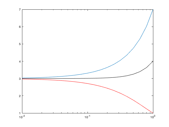
The resulting plot looks a lot like Figure M3.1.
Notice the tricks we've used:
1. The plot is logarithmic in the x-axis. This is done by using the
semilogx
command. This command works just like "plot", but scales the x-axis logarithmically.
2. The delta values we have defined are not evenly spaced - rather, their logarithm is evenly spaced. This is done so that we can uniformly cover two orders of magnitude in the stepsize.
We can also use the for loop to compute the derivative at many points. Let's consider finding centred difference approximations of
f(x) = x^3
between x = 1 and x = 3, with a stepsize delta = 0.25. We can do this as follows:
clear all

delta = 0.25;
x = 1:delta:3;
xp = x+delta;
xm = x-delta;
dfdx = (xp.^3-xm.^3)/(2*delta);

plot(x,dfdx)
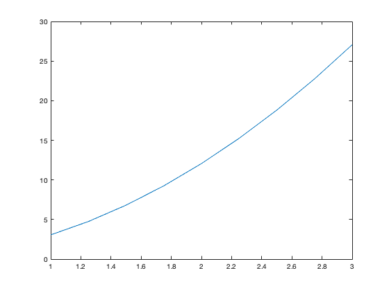
Note that we didn't have to use a for loop in this calculation. Neither did we have to use a for loop in the previous calculation over a range of different delta values. There is often more than one way to do a calculation.
How good is this approximation? Well - we know that
df/dx = 3x^2
We can plot this on the same figure.
dfdx_true = 3*x.^2;
hold on
plot(x,dfdx_true,'r')
hold off
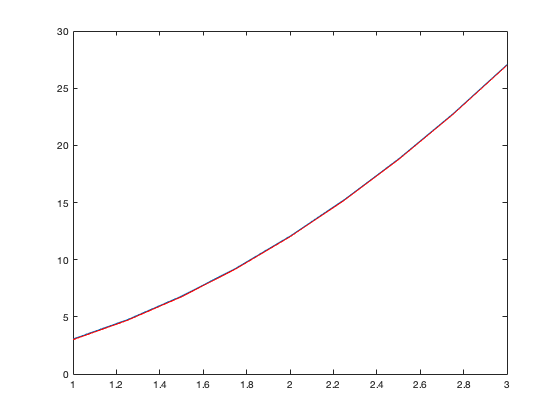
In fact, for this small value of delta, the agreement is excellent.
Now suppose that instead of knowing the function f(x) you want to approximate the derivatives of, you only have discrete values of f and x, such as:
x = (2, 2.5, 3, 3.5, 4, 4.5, 5)
f = (5.57, 9.88, 15.59, 22.92, 32.00, 42.96, 55.90)
If you want to approximate df/dx as a function of x, these discrete data is the only information you have. Suppose that what you want is an centred difference estimate of df/dx at each value of x you have been given data for. In this lab, we will assume that the values of x that you have been provided are evenly spaced (so the step size is uniform).
Thw following code can be used to approximate the values of the derivative using the centred difference approximation:
clear all

x = [2 2.5 3 3.5 4 4.5 5];
f = [5.57 9.88 15.59 22.92 32.00 42.96 55.90];

N = length(x);
delta = x(2)-x(1); % the step size in x

for k=1:N
    if (k==1)
        dfdx(k) = nan;
    end
    if (k==N)
        dfdx(k) = nan;
    end
    if ((k>1)&(k<N))
        dfdx(k) = (f(k+1)-f(k-1))/(2*delta);
    end
end

dfdx
dfdx =

       NaN   10.0200   13.0400   16.4100   20.0400   23.9000       NaN
Having defined the arrays x and f based on the data we were given, we then calculate the number of points N in these arrays and the stepsize delta that will be used in approximating the derivative. We then step through all values of x and compute our approximations, saved in the array dfdx. Once the loop has finished running, the values in the array dfdx are written to screen.
Note that the centred differences aren't defined at the end points (because we'd need points before and after the end points, which we don't have). So we only can estimate the derivative from k=2 to k=N-1. In the array dfdx, the end points have been assigned the value "nan", which stands for "not a number" - it's MATLAB's way of blanking out the value of an array element.
To make this calculation, we've introduced a new concept: the conditional statement. This occurs in the two blocks of code beginning with
if
and ending in
end
We'll talk about how this works in detail in a minute.
Conditional Statements
In the previous example, we made use of a conditonal statement. These allow you to have a program do different things in different circumstances. For example, in the above, different rules were used to assign values to elements at the beginning and end of the array dfdx than were used for all other elements.
The general form of a conditional statement is
if (condition)
things to do if condition is true
end
When the program encounters a block of code like this, the first thing it does is see if the condtion is satisfied. If it isn't, then this block of code (between "if" and "end") is ignored. If the condition is satisfied, then the block of code between the "if" and "end" statements is executed.
For example:
for k=1:5

    if (k>3)
        k
    end

end
k =

     4


k =

     5
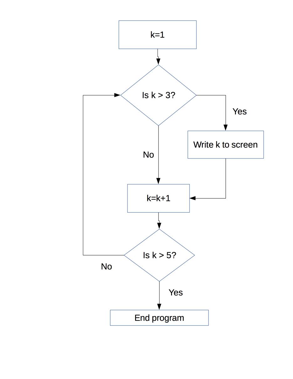
The way to read this code is: run the variable k from 1 to 5. If k is greater than three, then print k out to the screen. In fact, just what we see - nothing happens for k=1, 2, or 3, but k=4 and k=5 are printed out. A flow chart describing this code is as follows:
Another example:
x = -3:3;

for k=1:length(x)
    if (x(k)<0)
        y(k) = -x(k);
    end
    if (x(k)>=0)
        y(k) = x(k);
    end
end
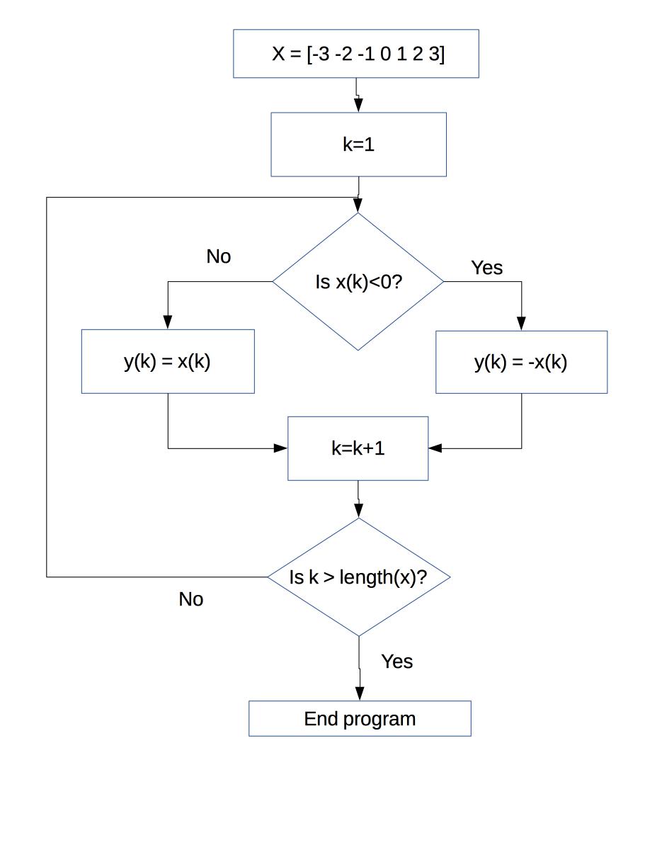
This code takes the integers between -3 and 3 and writes them to a new array, y. The kth value of y is x(k) if it is positive, and -x(k) otherwise. That is, this code computes the absolute value of x over this range. To see that this is what it's done compare
x
x =

    -3    -2    -1     0     1     2     3
with
y
y =

     3     2     1     0     1     2     3
A flowchart describing this code follows
The conditions we'll consider involve comparing two numbers: e.g. is the first bigger than the second? Are they equal? This comparison is done using the so-called "relational operators":
a == b  'a is equal to b'
a > b   'a is greater than b'
a < b   'a is less than b'
a >= b  'a is greater than or equal to b'
a <= b  'a is less than or equal to b'
a ~= b  'a is not equal to b'
Note the syntax of the first relational operator:
a == b
This compares the variables (or numbers) a and b to see if they have the same value. The meaning of this statement is fundamentally different from the statement
a = b
This statement doesn't compare the value of two variables: it sets the value of the variable a equal to the value of the variable b. For this to make sense, b must already have a value. When comparing two variables to see if they're equal, you need to use this "double equal sign" notation. For this operation to make sense, both a and b must already have values.
For example:
for k=1:5
    if (k==3)
        y = k^2
    end
end
y =

     9
When k is equal to 3 in the loop, the variable y is assigned the value k^2 (that is, 9).
With a slight change in the condition, we end up with a totally different answer:
for k=1:5
    if (k~=3)
        y = k^2
    end
end
y =

     1


y =

     4


y =

    16


y =

    25
In this example, y is assigned to k^2 for all values of k EXCEPT k=3 (remember that the "~=" operator means "does not equal").
Numerical Integration
We'll now carry on looking at how we can use these various tools to carry out numerical integration.
Let's consider Example M3.3, starting with the starting point approximation.
Type the following:
delta = 0.4;
x = 2:delta:4;
f = x.^3;

int = 0;
for k=1:length(x)-1
    int = int+f(k)*delta;
end
Notice what we've done here. The numerical integral involves adding a sequence of numbers; we've defined the variable "int" as the running tally. The syntax for this is straightforward: at each step in the loop, the running tally is updated by adding the new term in the sum. Remember that the line of code
a = a+b
is to be understood as "take the present value of a, add b to it, then assign the value of the sum to the variable a". When the loop is done, the final sum is the answer. For this approach to work it's very important to make sure that the running tally is zero before the loop begins - just what we've done in the line before the loop. Before anything has been added to the running tally, the running tally's value is zero. Note further that we're adding from the first element of x to the second-last. This is because we're using the starting-point approximation.
The blank line between the 2nd and 3rd lines of code isn't necessary - it's just there to make the code easier to read.
What's the value we get for the integral? Well,
int
int =

   49.2800
just like we saw in the notes.
To compute the end-point approximation all we need to do is type
delta = 0.4;
x = 2:delta:4;
f = x.^3;

int = 0;
for k=2:length(x)
    int = int+f(k)*delta;
end
All we've done is changed the first line of the loop statement - but this is an important change. The sum is now from the second to the last element of x. What do we get?
int
int =

   71.6800
Completely equivalently, we could take the for loop for this end point approximation from k=1 to k=length(x)-1, if we evaluate the function at the index value k+1 in each step of the loop:
delta = 0.4;
x = 2:delta:4;
f = x.^3;

int = 0;
for k=1:length(x)-1
    int = int+f(k+1)*delta;
end

int
int =

   71.6800
Finally, to get the trapezoidal approximation:
delta = 0.4;
x = 2:delta:4;
f = x.^3;

int = 0;
for k=1:length(x)-1
    int = int+(f(k)+f(k+1))*0.5*delta;
end

int
int =

   60.4800
Of the three approximations, the trapezoidal is the best (remembering that the true value of the integral is 60).
How do we get a figure like M3.7? Type the following script (best done in an M-file so you can easily correct typos):
N = 5:250;

for j=1:length(N)
    delta(j) = (4-2)/N(j);

    x = 2:delta(j):4;
    f = x.^3;

    int_s(j) = 0;
    int_e(j) = 0;
    int_t(j) = 0;

    for k=1:length(x)-1;
        int_s(j) = int_s(j)+f(k)*delta(j);
        int_e(j) = int_e(j)+f(k+1)*delta(j);
        int_t(j) = int_t(j) + 0.5*(f(k)+f(k+1))*delta(j);
    end

end

semilogx(delta,int_s)
hold on
semilogx(delta,int_e,'r')
semilogx(delta,int_t,'k')
hold off
axis([0.04 0.4 50 75])
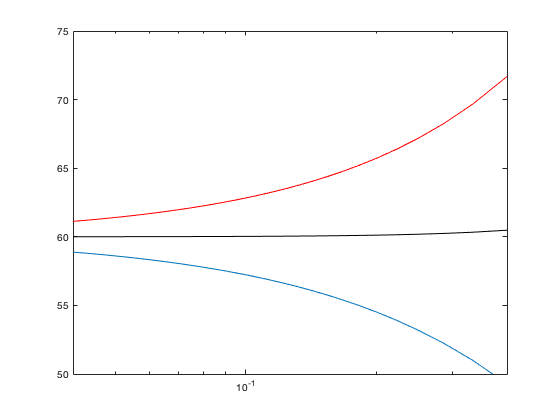
We have used a few new ideas here - the most important of which is that of "nested loops".
Remember that for the integrals above we've used loops to compute the running tally. That was for a single value of the stepsize delta - but what happens when you want to see results for a range of different stepsizes? Well - you loop through the stepsizes, and each step in this outer loop has another loop within it for the 3 integrals. This is known as "nesting". Each step of the outer loop - indexed by j - is just like the code we had above for doing the integral at a given value of delta. For j=1, we use delta(1) as the stepsize and calculate the approximations to the integral. Then the outside loop advances to j=2 and the approximations are evaluated for a stepsize delta(2) - and so on for all of the values of j in the outer loop. By having the outer loop, we can tell MATLAB to do the calculation for lots of values of delta.
Something that is very important to keep in mind with nesting loops is that you need to make sure that the variable names used for the indices in the inner and outer loops are different. If we'd used "j" as the index for the inner loops, MATLAB would become very confused - so we've used "k".
Now look at how we've set up the outer loop. In order to make sure that there are an integer number of steps between x=2 and x=4, we haven't specified the range of delta values for the outer loop - instead, we've specified the number of steps in the discretisation - in an array we've called "N" . Looping through the N array (this is the outer loop, indexed by j), first there are 5 steps , then 6, then 7 ... all the way up to 250 of them (you can see why we don't want to have to do these calculations by hand).
At each step j in the big loop, we need to figure out a value of delta corresponding to the number of steps N(j).
Consider the case delta = 0.4: then the x values are
x = 2.0, 2.4, 2.8, 3.2, 3.6, 4.0
It takes 5 steps of size 0.4 to get from x=2 to x=4, so the number of points in the discretisation is 1+5 = 6 - where we've had to remember to include the first point as well.
In general, it will take N steps of size delta to get from x to x+N*delta. Associated with those N steps will be N+1 points: the first point, and the points at the end of each of the N steps. Thus, the number of points will be one fewer than the number of steps. So if we know the beginning and end points ("a" and "b" respectively), and the number of steps "N" that we want, it follows that
delta = (b-a)/N
just like what we wrote in the code.
For each value of the big loop, we've saved values of delta, int_s, int_e, and int_t in arrays - so when the program is done running, we can plot these arrays.
The last line of code just makes the plot look better - it specifies the range of x and y coordinates that will be used in the plot. The syntax is
axis(["min x" "max x" "min y" "max y"])
(of course without the quotation marks). To see what it does, type
axis([0.04 0.4 30 95])
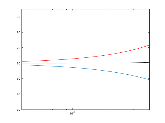
The vertical axis displayed is changed while the horizontal axis remains the same.
Exercises
Exercise 1
Write a program that plots the centred difference approximation to the derivative of the function
y = 3*(x^2)*exp(-x)
between x = 1 and x = 4 with stepsize delta = .25. On the same graph plot the exact derivative over this domain.
Exercise 2
Consider the dataset for the height of topography in an orogen at different times:
t (Myr) 0 0.25 0.5 0.75 1.0 1.25
h (km) 1.2 1.6 1.8 1.9 1.95 1.97
Estimate dh/dt for these various times using a centred difference approximation.
Plot h(t) against dh/dt. Based on this plot, can you rule out a model like Eqn. (2.4) in which the erosion rate depends linearly on h?
Exercise 3
Write a program that adds the numbers 1 to 8 excluding the number 6.
Exercise 4
Write a program that computes the trapezoidal approximation to the integral of
y = 2x-x^2
between x = 0 and x = 2 . First use the stepsize delta = 0.5, and then delta = 0.1. How does the error in the numerical approximation change as you change the stepsize? How do your numerical approximations compare to the true value of the integral?
Exercise 5
Plot the function
y = sin(2 pi x)   if   sin(2 pi x) > 0
y = 0             if   sin(2 pi x) <= 0
for x from 0 to 4.
Then compute the trapezoidal approximation of the integral of y(x) between x = 0 and x = 4 using a stepsize of delta = 0.1. Compare this approximation to the true value of the integral.
Exercise 6
Repeat Exercise 4 for the function
y = 2x-x^2 if 2x-x^2 > 0
y = 0 if 2x-x^2 <=0
Exercise 7
Consider the array
x = [0.2 1.6 1.1 0.5 2 0.8 1.2 1.2 0.1]
Write a program that extracts all elements greater than one from this array and writes these values into a second array. HINT: The second array will have a different number of elements than the first array. Before writing the code, determine by hand what the new array should be - and think about the process of filling in the new array sequentially, starting from the beginning of the array x.