Working with data in MATLAB

Reading and saving data
Working with data
Exercise 1
Exercise 2
Exercise 3

Reading and saving data

Suppose that you have carried out a large computation with MATLAB - one that takes a couple of hours or so to finish. Do you need to run this program every time you want to look at the output? No, you don't - not if you've saved the output to a file.

MATLAB provides many different options for saving data to a file, in many different formats using commands such as

fprintf

fwrite

These commands produce data files that can be read into MATLAB or into different programming languages; detailed descriptions of how to work with them can be found using the help command.

The easiest data format to work with in MATLAB -- and the one we'll focus on -- is MATLAB's own native format. Files in this format end with the ".mat" suffix - e.g.

data_out.mat

To save data in the .mat file 'flnm.mat', the command

save flnm.mat

is used. To retrieve data from the .mat file 'flnm.mat', the command

load flnm.mat

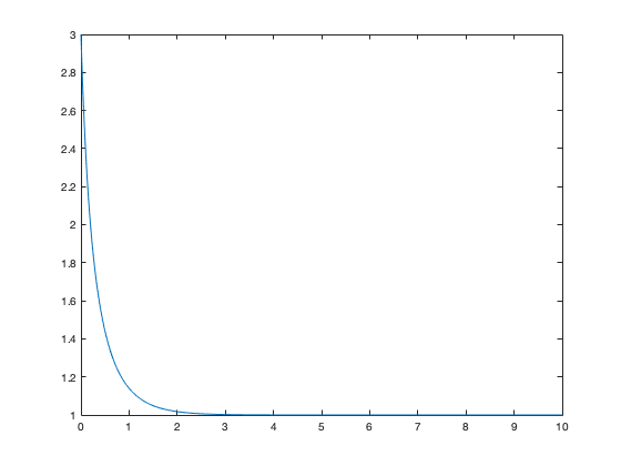
is used. Consider the following example, in which we numerically approximate the solution to an ODE

dt = .01;
t = 0:dt:10;

x(1) = 3;

for k=2:length(t)
    x(k) = x(k-1)+dt*(1-x(k-1)^2);
end

We can look at the solution:

plot(t,x)

To save the output to the file data1.mat we type

save data1.mat

We can then clear memory

clear all

If we now try to plot x against t, we'll get an error message - because neither is in memory:

plot(t,x)

Undefined function or variable 't'.

But if we load the data back into memory

load data1.mat

then both of the arrays x and t are back in memory

plot(t,x)

Being able to save to and read from data files is very important when working with programs that take a long time to run (so you don't want to have to do it over and over again), or when working with large datasets.

Working with data

Suppose we've measured the POC concentration in ocean sediments at a number of different depths and we want to estimate the surface sediment flux and refractory POC concentration, knowing that the bioturbation diffusivity is

D = 35 cm^2/kyr

that the remineralization rate coefficient is

k = 1.5x10^-9 s^-1

and that the burial flux rate w is negligible. As we discussed in section 6.5, we can do this using linear regression modelling.

But what are our data? Well, the data file

poc_data.mat

contains measurements of POC (in units mol/m^3) at depths z (measured in m) with the sign convention that z increases with depth. These data are saved in the arrays C and z. This dataset can be downloaded from the course website at

http://web.uvic.ca/~monahana/eos225/poc_data.mat

Download this file to your home directory. Having downloaded the data, let's read them in to MATLAB

load poc_data.mat

and have a look at them

plot(C,z,'o')

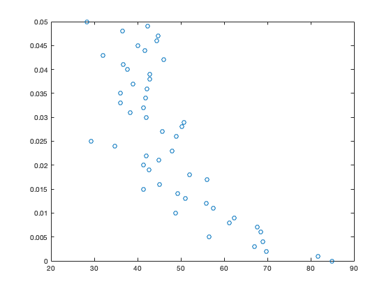
Note that because z increases with depth, deeper values of C are at the top of the plot. We can use the following command to flip the orientation of the plot

set(gca,'ydir','reverse')

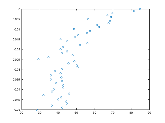
The set command can be used to change the plot in all sorts of ways - in this case, to set the y direction ('ydir') from 'normal' to 'reverse' (that is, increasing downward). To get more information, you can type

help set

These data show a general decrease of POC concentration with depth (as expected), but one which is noisy.

From our discussion in class, we know that we can write the POC profile predicted from the steady-state POC budget as the linear regression model

y = ax + b

with

y = C
x = (1/sqrt(D*K))*exp(-sqrt(k/D)z)
a = Phi
b = C_r

To estimate a and b, we'll need to compute some statistics. These computations involve adding up lots of numbers. Such sums are done easily in MATLAB when data is stored as 1xN arrays using the 'sum' command:

sum(M)

which simply adds up all of the elements in the 1xN array M. E.g. with

M = [1 3 8]

M =

     1     3     8

then

sum(M)

ans =

    12

is just the sum 1+3+8 = 12.

To carry out our statistical analysis, type the following in a text editor and save as poc_stats.m

load poc_data.mat

N = length(C);

D = 35/((100^2)*(1000*365*24*3600)); %% change D from cm^2/kyr to m^2/s
k = 1.5e-9;

y = C;
x = exp(-sqrt(k/D)*z)/sqrt(k*D);

mu_x = sum(x)/N;
mu_y = sum(y)/N;

sig_x = sqrt(sum((x-mu_x).^2)/(N-1));
sig_y = sqrt(sum((y-mu_y).^2)/(N-1));

rho = sum((x-mu_x).*(y-mu_y))/((N-1)*sig_x*sig_y);

a = (sig_y/sig_x)*rho;
b = mu_y-rho*sig_y*mu_x/sig_x;

Cr = b;
Phi = a;

Looking at a scatterplot of x with y:

plot(x,y,'o')

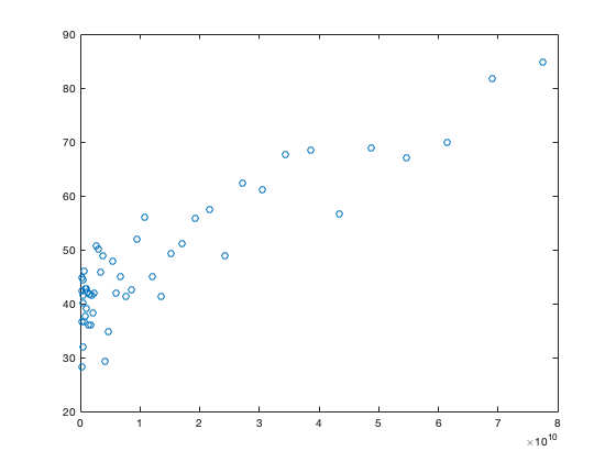
we can compare this to the line predicted by the regression model:

y_reg = a*x+b;

hold on
plot(x,y_reg,'r')
hold off

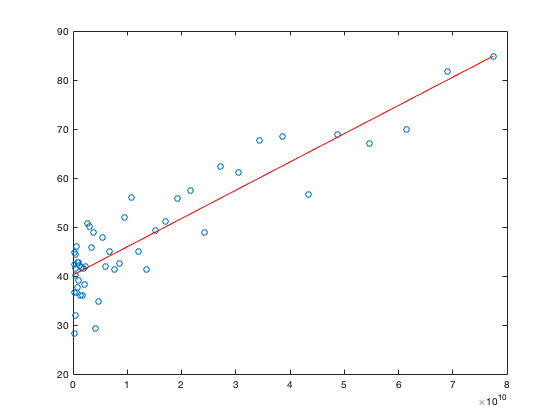
and we see that the regression model does a pretty good job of characterising the scatter of data. The fraction of variance of y "explained" by the regression is

rho^2

ans =

    0.8168

and the predicted values of the surface POC flux (in mol m^-2 s^-1) and concentration of refractory POC (in mol m^-3) are

Phi
Cr

Phi =

   5.7693e-10


Cr =

   40.2022

To get Phi in mmol m^-2 day^-1 we have

Phi*1000*24*3600

ans =

    0.0498

We can also look at plots not of x against y, but of z against C for both the data and the regression fit. Having computed estimates of Phi and Cr, we have all of the parameters necessary to plot our function C(z).

C_pred = Cr+(Phi/sqrt(k*D))*exp(-sqrt(k/D)*z);
plot(C,z*100,'o'),hold on
plot(C_pred,z*100,'r'),hold off
set(gca,'ydir','reverse')
xlabel('C (mol m^{-3})')
ylabel('z (cm)')

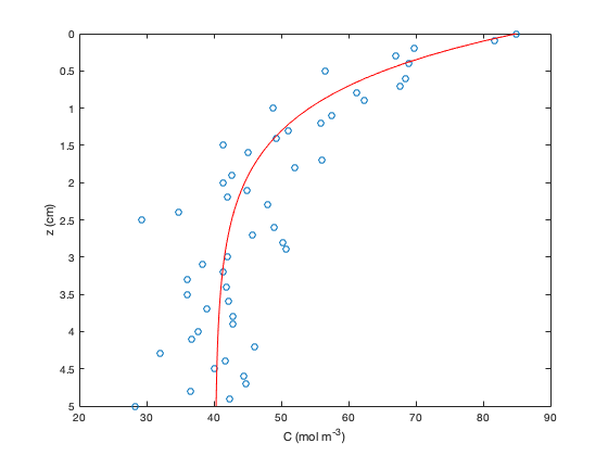
Note that we were able to get a superscript in the x label by typing '^{-3}'. The caret indicates that everything in the curly brackets is in superscript.

Exercise 1

Consider the dataset:

  x         y
 -8.6     -3.7
  6.6     -4.3
 -6.0     -8.4
 10.0      7.4
  0.13    -1.3
 -4.4      0.80
 -3.1     -7.1
 -5.2     -7.5
-12.3     -8.2
-10.3    -25.2

Assuming the linear regression model y = ax+b, determine least squares estimates of a and b. Plot both the original data and the regression line on the same figure. What fraction of the variance of y is accounted for by this regression?

Exercise 2

Repeat the estimates of Phi and Cr from the dataset poc_data.mat, using data from only the upper 2 cm. How do your estimates change?

Exercise 3