Numerical Approximation to Solutions of Differential Equations

A first example
Global radiative energy budget
Exercise 1
Exercise 2
Exercise 3
Exercise 4
Exercise 5
Exercise 6
Exercise 7
Exercise 8

A first example

We will now combine the various programming techniques we've learned with our understanding of numerical approximations of differential equations to write computer programs to compute approximate solutions of these equations.

Let's start with the ODE from example M4.1

dy/dx = y     y(x=0) = 1

with exact solution

y(x) = exp(x)

Having discretised x so that

x_n = x_0+n*delta

(where the underscore denotes a subscript) the forward-Euler approximation gives us the iteration

y_n = y_(n-1)+delta*y_(n-1)

We'll write a program that computes the forward-Euler approximation to the solution of this ODE from x = 0 to x = 10.

Type the following program into the new M-file ode_ex_1.m

% ODE example 1

delta = 0.1; % define stepsize
x_start = 0; % define starting value of x
x_stop = 10; % define stopping value of x

x = x_start:delta:x_stop; % define array x

y(1) = 1; % set initial condition

N = length(x);
for k=2:N
 y(k) = y(k-1)+delta*y(k-1);
end

y_true = exp(x);

plot(x,y),hold on
plot(x,y_true,'r'),hold off

Now run the program:

ode_ex_1

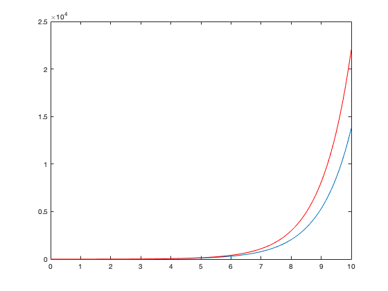
The plot shows both the exact and approximate solutions. Confirming the numbers reported in class,

  x(101)

ans =

    10

  y(101)

ans =

   1.3781e+04

that is, the approximation takes the value y=13.8e3 for x=10.

Let's dissect this code. We first defined three variables: the stepsize, the starting point for x, and the ending point for x. We then defined x as the array

x = x_start:delta:x_stop

Note that the first element of x - what we've called x_0 up to this point - is called x(1) by MATLAB. Remember that MATLAB indices must always be positive - there is no array element x(0). We always need to think carefully when translating a recipe like the forward-Euler method to a MATLAB program in order to get the indices correct.

We then define the initial condition by assigning the value 1 to the first element of a new array, y. Remember that y(1) is the first element of the y array. In terms of the function y(x) we are approximating, y(1) is the value of y corresponding to x(1).

Then, we define the number of points N in our approximate solution array. This is simply equal to the length of the array x, so we've used the length command to define N.

Remember that if the arrays x and y each have N elements, then the number of steps in the iteration is N-1. It takes N-1 steps to get from the first point to the Nth point.

Having done this, we're ready to implement the forward-Euler algorithm - which is expressed as a for loop. This shouldn't be surprising - remember the way in which this algorithm works. Starting from the approximation y(n-1), it tells us how to get y(n). So we start with y(1) to get y(2), use this result to get y(3), use this for y(4), and so on .... until we get to y(N).

Finally, we compute the exact solution (which in this case we know) and plot this and the approximate solutions on the same curve.

All we've done here is express in a computer program the iteration we worked out by hand in class. The above program could be used as the template for the computation of the forward-Euler to any ODE.

Having saved the program as an M-file allows us to easily change parameter values. For example, reduce the stepsize delta by a factor of 10 to

delta = 0.01;

and save the resulting program as ode_ex_2.m. Running this program (after first "clearing all"):

clear all
ode_ex_2

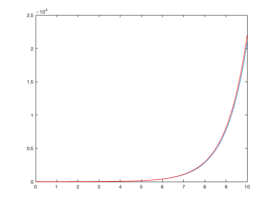
we obtain a new forward-Euler approximation, one which is closer to the exact solution (as we'd expect for a reduced stepsize). For the previous stepsize we had N = 101; now it is N=1001. This is not a calculation that we could easily have done by hand.

We can also modify the program ode_ex_1.m to compute the predictor-corrector approximation to the ODE (as in Example M4.3). In this case, all we need to do is change the iteration to:

for k=2:N
     ystar = y(k-1)+delta*y(k-1);
     y(k) = y(k-1)+0.5*delta*(y(k-1)+ystar);
end

Save the new program as ode_ex_3.m. Running this:

clear all
ode_ex_3

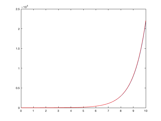
This approximation is even better than the forward-Euler with delta = 0.01, but has taken one fifth as many calculations to compute (a factor of 10 decrease for stepsize with a factor of 2 increase for predictor-corrector algorithm).

As a second example of using the predictor-corrector method, consider the ODE

dy/dx = x(1-y)    y(x=0) = 0;

with solution

y(x) = 1-exp(-(x^2)/2)

Remembering the generic form of a first-order ODE

dy/dx = f(x,y)

in this case we have

f(x,y) = x(1-y)

and so the code to compute the predictor-corrector approximation of the solution from x = 0 to x = 5 with stepsize delta = 0.1 is

clear all

delta = 0.1;
x = 0:delta:5;

y(1) = 0;
for k=2:length(x)
    f1 = x(k-1)*(1-y(k-1));
    ystar = y(k-1)+delta*f1;
    f2 = x(k)*(1-ystar);
    y(k) = y(k-1)+.5*delta*(f1+f2);
end

y_true = 1-exp(-.5*x.^2);

plot(x,y)
hold on
plot(x,y_true,'r')
hold off

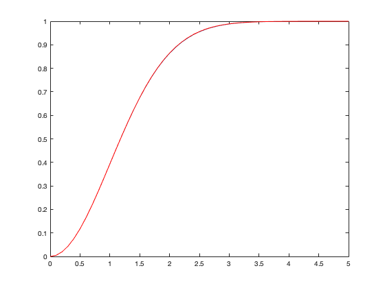
This code also plots the approximate and true solutions. Clearly, the approximate solution to the differential equation is close to the true solution. Note that in applying the predictor-corrector approximation, we evaluate the function f(x,y) twice: f(x(k-1),y(k-1)) and f(x(k),ystar). These two function evaluations have been put on separate lines and saved in the variables f1 and f2 respectively. It is not necessary to compute separate variables f1 and f2, but it makes the code easier to read (the lines are shorter and there aren't so many brackets within brackets).

Global radiative energy budget

Let's consider a more realistic example: the global radiative energy budget.

Suppose we consider the model from Secton 3.2, in which the surface temperature is approximated as constant while the atmospheric temperature evolves according to Eqn. 3.38. We will also assume that the surface is in radiative energetic equilibrium, so Ts is given by Eqn. (3.28). With albedo alpha=0.3, emissivity epsilon=0.77, and solar energy density Is=1367 W/m2 we get the equilibrium atmospheric temperature (Eqns 3.26 and 3.28):

Taeq = (Is*(1-alpha)/(8*sigma*(1-epsilon/2))^.25

Taeq = (1367*(1-0.3)/(8*5.67e-8*(1-.77/2)))^.25

Taeq =

  242.0079

so the equilibrium atmospheric temperature is 242 K. Now - starting away from equilibrium, how does the temperature change? For small displacements from equilibrium, we used a linearised approximation to address this question. What about when the anomaly is not small - say, an initial temperature T(t=0) = 300 K giving the anomaly T'(t=0) = 58 K? To see how the system changes from this initial condition, we'll have to use numerical methods to solve the full equation:

dTa/dt = (g/(c*ps))*2*epsilon*sigma*[Taeq^4 -Ta^4]

Type the following program into the text editor and save as the program atmos_energy_1.m:

% atmospheric energy budget

% set model parameters

sigma = 5.67e-8;
Taeq = 242;
epsilon = 0.77;
c = 1000;
g = 9.81;
ps = 1e5;

% define time (in seconds)

dt = 5*24*60*60;
t0 = 0*24*60*60;
t1 = 200*24*60*60;
t = t0:dt:t1;

Ta(1) = 300; % initial condition

N = length(t);
for k=2:N
    Ta(k) = Ta(k-1)+dt*(g/(c*ps))*(2*epsilon*sigma)*(Taeq^4-Ta(k-1)^4);
end

plot(t,Ta)

Running the program:

clear all
atmos_energy_1

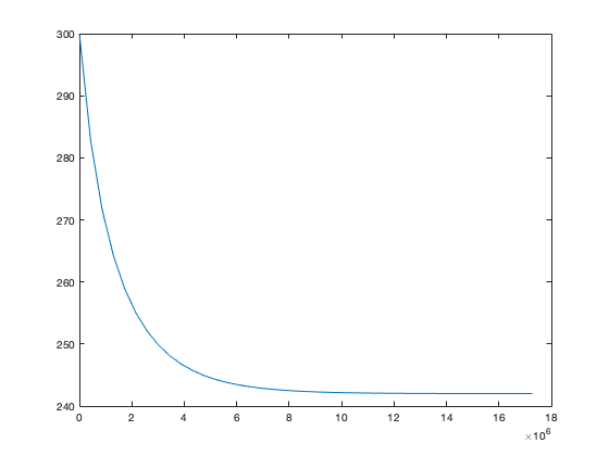
Note that because we've defined all of our parameters in terms of MKS units (metres, kilograms, seconds etc.) we have to make sure that time is also defined in seconds.

As expected, starting from the initial condition at T=300K, the system temperature decreases and approaches equilibrium.

Remember the linearised model predicted that

Ta(t) = Taeq + Ta'(0)exp(-t/tau_a)

where

tau_a = (c*ps/(8*g*epsilon*sigma*Taeq^3)) = 2.06 x 10^6 s = 24.1 days

How does this linearised approximation compare to the full nonlinear solution? Defining:

Ta_lin = 242+58*exp(-t/2.06e6);

Plotting this on the same plot as the full solution:

hold on
plot(t,Ta_lin,'r')
hold off

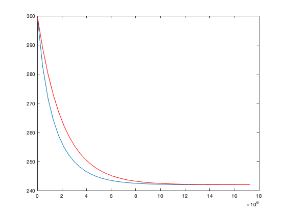
we see that the full nonlinear solution approaches equilibrium faster than what would be predicted by the linearised approximation (which remember we don't expect to be particularly good because the initial perturbation isn't "small").

We do expect the linearised approximation and the full nonlinear solution to be in closer agreement when the initial perturbaton is small. Change the initial condition in atmos_energy_1.m to

T(1) = 245;

so the initial anomaly is T'(t=0)=3 K, and save the resulting program as atmos_energy_2.m. Running this:

atmos_energy_2

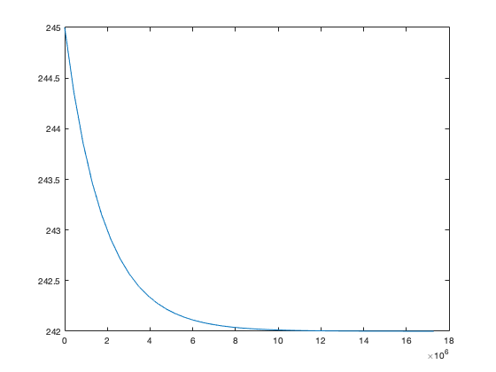
We then have

T_lin = 242+3*exp(-t/2.06e6);
hold on
plot(t,T_lin,'r')
hold off

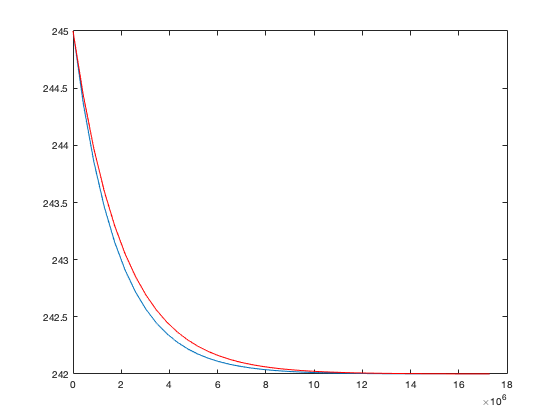
For the smaller initial perturbation, the linear approximation is in closer agreement with the fully nonlinear soluton.

Now - what about the model in Example 3.3, for which the albedo is a function of the surface temperature Ts and Ta is assumed to adjust instantaneously to Ts? How were the computational results in this Example produced?

First, let's reproduce Figure 3.9. Type the following into the text editor and save it as fig3_9.m

Ts = 225:1:300;
sigma = 5.67e-8;
epsilon = .77;
Is = 1367;
alpha_min = .3;
alpha_max = .7;
T1 = 245;
T2 = 275;

Fout = (1-epsilon/2)*sigma*Ts.^4;

for k=1:length(Ts)
 if (Ts(k)<=T1)
     alpha = alpha_max;
 elseif ((Ts(k)>T1)&(Ts(k)<=T2))
     alpha = (alpha_min-alpha_max)*(Ts(k)-T1)/(T2-T1)+alpha_max;
 elseif (Ts(k)>T2)
     alpha = alpha_min;
 end
 Fin(k) = Is*(1-alpha)/4;
end

plot(Ts,Fout)
hold on
plot(Ts,Fin,'r')
hold off

Running this program:

clear all
fig3_9

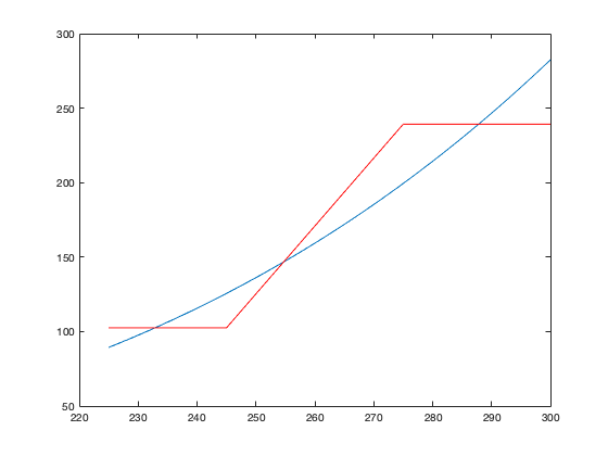
Zooming in on the crossing points, where Fin equals Fout, we can read off the values of the three equilibrium temperatures.

We've done a couple of new things in this program. First, we've used a somewhat more complicated conditional statement: instead of just a single possibility, we've allowed for three different cases:

Ts <= T1 or T1 < Ts <= T2 or T2 < Ts

These different possibilities have been coded as follows:

if (case A)
  action A
elseif (case B)
  action B
elseif (case C)
  action C
end

which is interpreted as follows:

if case A holds, then do action A

but if not

if case B holds, then do action B

but if not

if case C holds, then do action C

but if not

don't do any of actions A, B, or C.

This is a bit more complicated than a basic "if ... end" statement - but the fundamental logic is the same. In both cases, code like this allows MATLAB to decide between different courses of action depending on the value of some variable.

Also note how we've written the second condition:

(Ts(k)>T1)&(Ts(k)<=T2)

This case holds if the temperature Ts(k) is greater than T1 and less than or equal to T2. The "&" symbol between the two comparisons says that this case only holds if both statements are true. This is an example of a "relational operator", of which there are different kinds. You can get an idea of the different kinds of relational operators by typing "help relop".

We're now in a position to reproduce Figure 3.10 (for delta = 0.05 years). Type the following into the text editor, and save as fig3_10.m:

sigma = 5.67e-8;
epsilon = 0.77;
Is = 1367;
g = 9.81;
c = 4000;
H = 100;
rho = 1020;
alpha_min = .3;
alpha_max = .7;
T1 = 245;
T2 = 275;

delta = 0.05*24*3600*365;
tmin = 0*24*3600*365;
tmax = 50*24*3600*365;
t = tmin:delta:tmax;

T(1) = 260;
N = length(t);
for k=2:N
 if (T(k-1)<=T1)
     alpha = alpha_max;
 elseif ((T(k-1)>T1)&(T(k-1)<=T2))
     alpha = (alpha_min-alpha_max)*(T(k-1)-T1)/(T2-T1)+alpha_max;
 elseif (T(k-1)>T2)
     alpha = alpha_min;
 end

T(k) = T(k-1)+delta*((1/(c*H*rho))*(.25*Is*(1-alpha)-(1-epsilon/2)*sigma*T(k-1)^4));

end

plot(t/(24*3600*365),T)
axis([0 50 260 290])

Running the program:

fig3_10

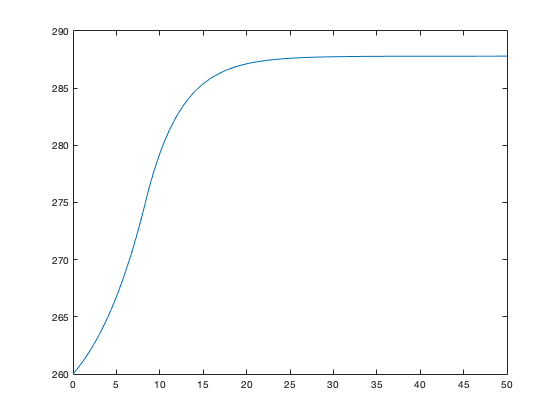
gives the curve shown in Figure 3.10, with surface temperature in Kelvin plotted as a function of time in years.

Exercise 1

Approximate the solution of the ODE

dy/dx = y(1-y) , y(x=0) = 0.25

numerically using both forward-Euler and predictor-corrector methods with delta = 0.05, from x = 0 to x = 10. Solve the ODE exactly, and plot the exact solution on the same plot as the numerical approximations.

Exercise 2

Repeat Exercise 1 for the ODE

dy/dx = xy(1-y) , y(x=0) = 0.25

Exercise 3

Rewrite atmos_energy_1.m to do the calculation using the predictor-corrector method rather than the Forward-Euler approximation.

Exercise 4

Rewrite fig3_10.m to compute numerical approximations for T(t) for delta = 5 years, delta = 0.5 years, and delta = 0.05 years, and plot these over top of each other (just like in Figure 3.10).

Exercise 5

Write a program to reproduce Figure 3.11, producing four curves T(t) for initial conditions T(t=0) = 220K, 240 K, 275 K, and 300 K.

Exercise 6

Consider an orogen for which the topograhic elevation evolves under the influence of crustal shortening and erosion (with a rate proportional to h), as discussed in Section 2.1. Suppose the erosional timescale is 1.5 million years, that the crustal shortening rate is 0.75 mm/yr, and that at t = 0 there was no topography. Numerically approximate the solution of the ODE for h(t) from Section 2.1 from t = 0 to t = 10 million years, using a forward-Euler approximation with stepsize 100,000 years. Make a plot of h(t) over this period.

Exercise 7

Returning to Exercise 6, suppose the crustal shortening rate stays constant at 0.75 mm/yr only for 10 million years. After that, the tectonic processes change and crustal shortening ceases. Find the numerical approximation of the solution the of ODE for h(t) from Section 2.1 from t = 0 to t = 20 million years, using a forward-Euler approximation with stepsize 100,000 years. Make a plot of h(t) over this period.

Exercise 8

Compute the forward-Euler approximation to the solution of the ODE

dB/dt = aB - B^2

from t = 0 to t = 30 using a stepsize delta = 0.01 and initial condition B(0) = 0.05, where

a = 1  if sin(2*pi*t) > 0
a = 0  if sin(2*pi*t) <= 0

An ODE such as this can arise when modelling the biomass of photosynthetic primary producers, taking the day/night cycle into account (no photosynthesis occurs at night).

Numerical Approximation to Solutions of Differential Equations

Contents

A first example

Global radiative energy budget

Exercise 1

Exercise 2

Exercise 3

Exercise 4

Exercise 5

Exercise 6

Exercise 7

Exercise 8